Neural network driven model discovery for physics

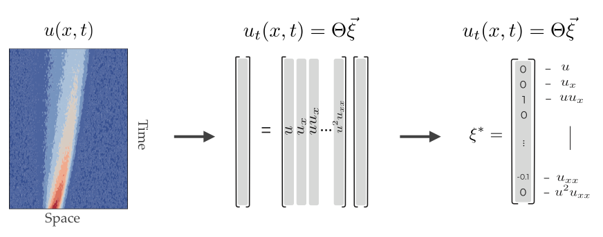
In this short blog post I will walk you through an example for neural network driven model discovery using the tool DeepMoD [1]. Essentially this tool allows the user to infer the differential equation underlying a spatio-temporal data set from a predefined set of library functions. This approach combines classical symbolic regression task with training a neural network to represent the data. Symbolic regression is a classical data-science approach that seeks the mathematical or physical expression that “fits” the presented data best. Knowledge of the underlying equations of a data-set allows for extrapolation of the data-set and interpretation of the physical/mathematical parameters involved in the problem at hand.

In this post we will apply DeepMoD to discover the 2D advection diffusion equation. We a PDE of the form,

The choice of the library function at the right hand side of the equation depend on the problem at hand, in this post we consider all permutations of derivatives up to second order and polynomial terms in u, up to second order, so 18 candidate terms in total.

To solve this task, DeepMoD employs a sparse regression algorithm by rewriting the problem as a simple matrix vector product:

where Θ is the library that contains the candidate terms evaluated on all the sample points and ξ is the coefficient vector which indicates which and to what extent the different candidate terms feature in the equation. It's this vector ξ that we try to discover.

Since we generally consider a extensive library Θ it is important to find a sparse version of the coefficient vector ξ, i.e., that the underlying PDE contains a limited amount of terms. The approach used in DeepMoD is to use a neural network to learn the mapping of the data, i.e. {x,t} →u, and then employ automatic differentiation to accurately calculate the derivatives of u with respect to x and t, which can then be used to construct Θ. By including the regression task within the cost function of the neural network, training the network not only adjusts the weights and biases of the network, but also adjusts the components of the coefficient vector ξ. Finally, an L_1 term on ξ is added to the cost function to ensure its sparsity. To summarize, training the neural network thus corresponds to optimizing the sum of these three contributions:

 In the remainder of this post we will apply this on a data-set of 2D advection diffusion.

Preparing the 2D advection diffusion data

First of all we import the DeepMoD package as well as some other essential python toolboxes. All the code shown here, and many more examples is available on https://github.com/PhIMaL/DeePyMoD_torch. 

import numpy as np
import matplotlib.pylab as plt
from scipy.io import loadmat
import torch

from deepymod_torch.DeepMod import DeepMod
from deepymod_torch.library_functions import library_2Din_1Dout
from deepymod_torch.training import train_deepmod

We start by importing the spatio-temporal data set of a 2D advection diffusion problem, where u is the density field which evolves over space {x,y} and time t:

data = loadmat('data/Advection_diffusion.mat')
sol = np.float32(data['Expression1']).reshape((51,51,61,4))

x = sol[:,:,:,0]
y = sol[:,:,:,1]
t = sol[:,:,:,2]
u = sol[:,:,:,3]

This data set corresponds to a advection diffusion problem with a diffusion coefficient of 0.5 and a drift of (v_x, v_y) = (0.25,0.5),

We combine all the input data into a single input vector X={t,x,y} and flatten the output vector U accordingly,

X = np.transpose((t.flatten(),x.flatten(), y.flatten()))
U = u.reshape((u.size, 1))

Next, to show the robustness of the algorithm w.r.t. elevated noise levels and a limited size of the data set, we add 10% white noise and sample 1000 data-points from the data set and combine all in an input tensor X_train and output tensor U_train,

noise_level = 0.1
U_noisy = U + noise_level * np.std(U) * np.random.randn(U.size, 1)
number_of_samples = 1000

idx = np.random.permutation(U.shape[0])
X_train = torch.tensor(X[idx, :][:number_of_samples], dtype=torch.float32, requires_grad=True)
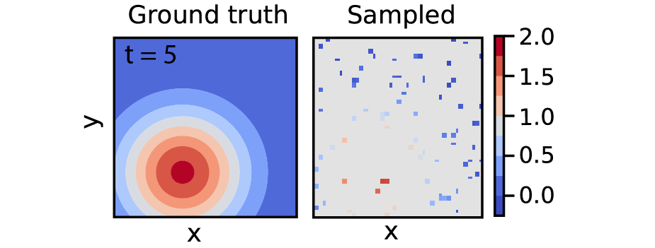
U_train = torch.tensor(U[idx, :][:number_of_samples], dtype=torch.float32)

Below we give an impression of the original data and the sampled data at a given time frame (of which we have 51):

Configure DeepMoD 

Nex’t up we will set the configurations of DeepMoD, 

## Configuration DeepMoD
config = {'n_in': 3, 'hidden_dims': [20, 20, 20, 20, 20, 20], 'n_out': 1, 'library_function': library_2Din_1Dout, 'library_args':{'poly_order': 2, 'diff_order': 2}}

So in this previous line we choose:

• n_in: Input dimension, which in our case is 3, considering one temporal and two spatial dimensions {t,x,y}

• hidden_dims: Architecture of the feed forward neural network, in this case we choose 6 layers of 20 neurons. For most of the cases we tested, the algorithm is insensitive to this choice as long as the amount of neurons is sufficient to learn the mapping (roughly O(100) neurons total)

• n_out: Output dimension, this is 1 in our case, the density u

• library_function: This is the name of a predefined library function that takes two spatial dimensions (+ time) as input and generates a library containing all the permutations of spatial derivatives (x and y) up to order ‘diff_order’ and polynomial terms up to order ‘poly_order’

To summarize we have set the architecture of the neural network and defined a library Θ which contains 18 different terms:

Next, we initialize the model with this configuration file and define the optimizer that we want to use. In this case we use an ADAM optimizer and set the learning rate for the weights of the neural network (‘model.network_parameters) as well as for update of the coefficient vector ξ (‘model.coeff_vector):

model = DeepMod(**config)

optimizer = torch.optim.Adam([{'params': model.network_parameters(), 'lr':0.001}, {'params': model.coeff_vector(), 'lr':0.005}])

Running DeepMoD 

Now that everything is in place we train the neural network for 30000 epochs by executing,

train_deepmod(model, X_train, U_train, optimizer, 30000, {'l1': 1e-5})

Note that in this last step we have to set magnitude of the L_1 penalty. Setting an L_1 penalty speeds up convergence and ensures we obtain a sparse solution with fewer epochs.

During the optimization we can follow the progress of the algorithm on the screen,

• The current epoch, progress and remaining time

• The total magnitude of the cost function composed of its three elements: the MSE (learning the mapping {t,x,y} →u), the regression task (finding the coefficient vector ξ and finally the L_1 penalty) 

In addition to this we can also follow the progress of the training (coefficient vector ξ and all the different losses) in a custom build tensor board file. The tensorboard files are automatically written in the /runs/ folder and can be acceded by running the following command in the command line,

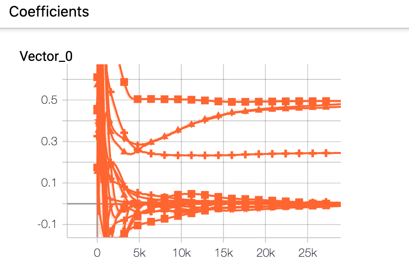
tensorboard --logdir=/runs/FOLDER_NAME

This tensorboard file shows us, among other metrics the evolution of the coefficient vector: 

This shows that after 30000k epoch, four terms of the vector ξ do not approach zero. These terms correspond to the two diffusion terms (u_xx and u_yy) as well as the advection term (u_x and u_y).

After DeepMoD has completed the 30000 epochs (<10min on a laptop) the elements of ξ that approach zero are thresholded (See further discussion in [1]):

Finally, a second run of DeepMoD is automatically launched with the remaining elements (u_xx, u_yy, u_x and u_y) and a vanishing L_1 penalty. This is to fine tune the remaining coefficients. We can now evaluate the final coefficients obtained by DeepMoD: 

print(model.fit.coeff_vector[0])
>> Parameter containing:
>> tensor([[0.2457],
        [0.4958],
        [0.4918],
        [0.4875]], requires_grad=True)

We note that we obtain a nearly perfect match with the ground truth for the advection vector (0.25, 0.5) and the diffusion coefficient (0.5, 0.5).  So finally DeepMoD discovered the correct equation as well as accurately estimated all the relevant coefficients.

Some final thoughts 

The example we present here considers a 2D PDE. In the examples folder: https://github.com/PhIMaL/DeePyMoD_torch we provide notebooks for a variety of PDEs and ODEs. When applying this to your own data sets it is important however to keep in mind the following points:

• While the size of the neural network does not seem to impact the results for most examples we considered, highly periodic function generally require more layers/neurons to effectively learn the mapping {x,t}→u, so in case the mse does not converge, increasing the amount of neurons could resolve the issue.

• The threshold implemented remains in some way arbitrary and we strongly advise to run a single run of DeepMoD first and inspect the resultant coefficient vector ξ and sparsity pattern carefully. Sometimes, an automatic threshold discards obvious non-zero elements. 

• As we show in some other examples in the Github repo, a custom build library containing non-linear terms such as sin(u) can easily be constructed within a notebook/script. This allows the user to add terms to the library that could be expected in the ODE/PDE

If in doubt or you have any questions, don’t hesitate to contact us directly through Github or Twitter (@GJ_Both or @RemyKusters).  

[1] Both, Gert-Jan, et al. “DeepMoD: Deep learning for Model Discovery in noisy data.” arXiv preprint arXiv:1904.09406 (2019).